Introduction
I will create a table with information about metropolitan areas in the United States. For simplicity, they will just be called “cities”. The variables are:
- Population,
- Average Rental Price,
- Median Rental Price,
- Unemployment Rate,
- Per Capita Income,
- Air Quality,
- Walk, Transit, and Bike Scores,
- Cost of Living,
- Price Parity,
- Median Commute Time,
- Latitude, Longitude.
I have divided this project into two parts.
Part I. After finding the data in open sources, I clean it if necessary and load it one by one with a simple custom function. Along the way, I explain the methodology for each metric and what it means. The data set can be found on this project’s GitHub page and on Kaggle.
Part II. The second part of the project is exploratory data analysis. I explore the variables I find most interesting and their relationship to each other through visualization and testing.
Expectations. A complete dataset with American cities and information about them. A demonstration of what can be done with this data for analysis and insights.
Loading Data
In this part we will create a DataFrame with the 14 columns mentioned above, explaining the meaning and methodology behind each one.
1
2
3
| # Import libraries used in this project
import numpy as np
import pandas as pd
|
Create an empty DataFrame and define a function to append new columns to it later.
1
2
3
4
5
6
7
| cities = pd.DataFrame(columns=['City', 'State'])
def merge_frames(new_df, method='left', print_ten=False):
df = pd.merge(cities, new_df, on=['City', 'State'], how=method)
if print_ten == True:
print(df.head(10))
return df
|
First Four Columns
Population
Metropolitan Area Population in 2020. Data from Census, retrieved from citypopulation.de and preprocessed by myself in Excel.
1
2
| pop = pd.read_csv('Data/population.csv')
cities = merge_frames(pop, method='right', print_ten=True)
|
1
2
3
4
5
6
7
8
9
10
11
| City State Population
0 New York NY 20140470.0
1 Los Angeles CA 13200998.0
2 Chicago IL 9618502.0
3 Dallas TX 7637387.0
4 Houston TX 7122240.0
5 Washington DC 6385162.0
6 Philadelphia PA 6245051.0
7 Miami FL 6138333.0
8 Atlanta GA 6089815.0
9 Boston MA 4941632.0
|
Average Rent
The average rent for a one-bedroom apartment. Data from Zillow.
Monthly averages are calculated by regressing changes in rental prices on the change in time between two transactions and adjusting the weights based on the prevalence of rented units. The index is then smoothed and denominated in dollars to make it easier to interpret.
1
2
3
4
5
| # Load data with rent means, assign columns names
cols = ['RegionName', 'StateName', '2023-01-31']
new_cols = ['City', 'State', 'AvgRent']
rent_means = pd.read_csv('Data/rent_mean_2023.csv', usecols=cols)
rent_means.columns = new_cols
|
1
2
3
4
| # Drop NaN values, change data types
rent_means = rent_means.dropna(how='any')
rent_means['City'] = rent_means['City']
rent_means.loc[:, 'AvgRent'] = rent_means['AvgRent'].apply(lambda x: int(x))
|
1
2
| # Append the average rent variable to the main DataFrame with a custom function
cities = merge_frames(rent_means, method='inner', print_ten=True)
|
1
2
3
4
5
6
7
8
9
10
11
| City State Population AvgRent
0 New York NY 20140470.0 3272
1 Los Angeles CA 13200998.0 2857
2 Chicago IL 9618502.0 1975
3 Dallas TX 7637387.0 1754
4 Houston TX 7122240.0 1620
5 Washington DC 6385162.0 2421
6 Philadelphia PA 6245051.0 1663
7 Miami FL 6138333.0 3201
8 Atlanta GA 6089815.0 1991
9 Boston MA 4941632.0 3419
|
Median prices for a one-bedroom apartment. Data from HUD User.
The 50th percentile rent estimates are based on the most recent data available from the American Community Survey, which is conducted by the U.S. Census Bureau. They are calculated using a model that takes into account geography, unit size, and lease type (e.g., rent-controlled vs. market rate).
1
2
3
4
5
| # Load data with rent means, assign column names, set delimiters
cols = ['hud_areaname', 'rent_50_1']
new_cols = ['City', 'MedianRent']
rent_medians = pd.read_csv('Data/rent_median_2023.tsv', usecols=cols, delimiter='\t')
rent_medians.columns = new_cols
|
1
2
3
4
5
6
7
8
9
10
11
12
| # Create a State column and clean up the city names
rent_medians['State'] = rent_medians['City'].apply(lambda x: x.split(',')[-1].strip()[:2])
rent_medians['City'] = rent_medians['City'].apply(lambda x: x.split(',')[0].split('-')[0])
# Remove the comma from MedianRent and make it an integer
def remove_comma(x):
if ',' in x:
return x.replace(',', '')
return x
rent_medians['MedianRent'] = rent_medians['MedianRent'].apply(lambda x: int(remove_comma(x)))
rent_medians.head(10)
|
| City | MedianRent | State |
|---|
| 0 | San Francisco | 3000 | CA |
|---|
| 1 | San Jose | 2763 | CA |
|---|
| 2 | Santa Cruz | 2602 | CA |
|---|
| 3 | Santa Maria | 2490 | CA |
|---|
| 4 | Boston | 2368 | MA |
|---|
| 5 | Salinas | 2324 | CA |
|---|
| 6 | New York | 2323 | NY |
|---|
| 7 | Stamford | 2321 | CT |
|---|
| 8 | Santa Ana | 2274 | CA |
|---|
| 9 | Dukes County | 2200 | MA |
|---|
1
| cities = merge_frames(rent_medians, print_ten=True)
|
1
2
3
4
5
6
7
8
9
10
11
| City State Population AvgRent MedianRent
0 New York NY 20140470.0 3272 2323.0
1 Los Angeles CA 13200998.0 2857 1925.0
2 Chicago IL 9618502.0 1975 1364.0
3 Dallas TX 7637387.0 1754 1440.0
4 Houston TX 7122240.0 1620 1216.0
5 Washington DC 6385162.0 2421 1740.0
6 Philadelphia PA 6245051.0 1663 1314.0
7 Miami FL 6138333.0 3201 1670.0
8 Atlanta GA 6089815.0 1991 1489.0
9 Boston MA 4941632.0 3419 2368.0
|
Unemployment
Unemployment Rates for Metropolitan Areas in January 2023, Not Seasonally Adjusted. Data from U.S. Bureau of Labor Statistics.
The unemployment rate is calculated as the number of unemployed individuals divided by the total labor force, which is the sum of employed and unemployed individuals. The unemployed are defined as individuals who are not currently employed but are available for work and have actively sought work in the past four weeks. Data are collected through a monthly survey of households called the Current Population Survey. The survey is conducted by the U.S. Census Bureau and is designed to be representative of the civilian, noninstitutionalized population 16 years of age and older.
1
2
3
4
5
6
7
8
9
10
11
12
13
14
15
16
17
18
19
20
21
22
23
24
25
26
| # The data in unemp.txt needs some cleaning,
# because the values are separated by not one, but three delimiters (tabs, commas, and newlines).
temp_list1 = []
temp_list2 = []
unemp_list = []
# Open text file with unemployment rate data.
# This file is broken, because every first value has a newspace character and every second has a trailing tab.
with open("Data/unemp.txt", 'r') as unemp:
for i, line in enumerate(unemp.readlines()):
# If line is even, add to the first temp_list
if i % 2 == 0:
# Clean the line and split cities and states
this_line = line.rstrip(' \n').split(', ')
# Leave only one city from metropolitan area and one state
city_state = [this_line[j].split('-')[0] for j in range(len(this_line))]
temp_list1.append(city_state)
# If line is odd, add to the second temp_list
else:
# We need onnly the rate variable
temp_list2.append(line.split('\t')[0])
# Create a final list from two temporary ones
for i in range(len(temp_list1)):
unemp_list.append(temp_list1[i] + [temp_list2[i]])
del temp_list1, temp_list2
|
1
2
3
| # Create an unemployment DF
unemp_df = pd.DataFrame(unemp_list, columns=['City', 'State', 'UnempRate'])
print(unemp_df.head(10))
|
1
2
3
4
5
6
7
8
9
10
11
| City State UnempRate
0 Madison WI 1.6
1 Columbia MO 1.7
2 Decatur AL 1.8
3 Fond du Lac WI 1.8
4 Huntsville AL 1.8
5 Logan UT 1.8
6 Sheboygan WI 1.8
7 Ames IA 1.9
8 Appleton WI 1.9
9 Columbus IN 1.9
|
1
| cities = merge_frames(unemp_df)
|
Last Ten Columns
The next set of variables come in a more tidy format and are simply appended to the main DataFrame. However, some of them were pre-processed by me in Excel to save time. In most cases, it was just a matter of splitting the columns by a certain delimiter and deleting unnecessary commas and dots in the numeric values.
Average Income
Per Capita Income by Metropolitan Area in 2021.Data from U.S. Bureau of Economic Analyses (pre-processed by myself in Excel).
Per capita income is calculated by dividing population by personal income. Total personal income includes all income received by all people in the area, including wages and salaries, proprietors’ income, rental income, and government transfer payments. Population estimates are based closely on data from the U.S. Census Bureau.
1
2
| income_personal = pd.read_csv('Data/income_personal.csv')
cities = merge_frames(income_personal)
|
Air Quality
Air Quality Index (AQI). Data from U.S. Environmental Protection Agency.
The AQI is based on concentrations of five major air pollutants regulated by the Clean Air Act: ground-level ozone, particulate matter, carbon monoxide, sulfur dioxide, and nitrogen dioxide. The AQI is calculated based on the highest concentration of these pollutants in a given area over a given period of time and then scaled to a value between 0 and 500.
An AQI less than 50 is considered good, from 51 to 100 - moderate. If the AQI is higher than 100, the air quality is unhealthy: first for certain sensitive groups of people, and then for everyone as the AQI gets higher and higher.
1
2
| air = pd.read_csv('Data/aqi.csv')
cities = merge_frames(air)
|
Walkability and Bike Score
Data from Walk Score.
Walk Score measures the walkability of an area. Points are assigned to each address based on the distance to amenities in each category. Amenities within a 5-minute walk receive maximum points. A decay function is used to award points to more distant amenities, with no points awarded after a 30-minute walk.
Bike Score measures how good a place is for biking. It’s calculated by measuring bike infrastructure (lanes, trails, etc.), hills, destinations and street connectivity, and the number of bike commuters.
Each score uses the same metric to translate itself into a description. Example with Walk Score:
- 90–100 Daily errands do not require a car (Walker’s Paradise)
- 70–89 Most errands can be accomplished on foot.
- 50–69 Some errands can be accomplished on foot.
- 25–49 Most errands require a car (car-dependent).
- 0–24 Almost all errands require a car (car-dependent).
1
2
| walkability = pd.read_csv('Data/walkscore.csv')
cities = merge_frames(walkability)
|
Transit Score
Data from AllTransit.
Transit Score measures access to public transportation. The Performance Score by AllTransit takes into account connections to other lines, jobs within a 30-minute transit commute, and the number of workers who use transit to get to work. It measures the performance on a scale of 0 to 10.
1
2
| transit_score = pd.read_csv('Data/transit_score.csv')
cities = merge_frames(transit_score, print_ten=True)
|
1
2
3
4
5
6
7
8
9
10
11
12
13
14
15
16
17
18
19
20
21
22
23
| City State Population AvgRent MedianRent UnempRate AvgIncome \
0 New York NY 20140470.0 3272 2323.0 3.8 85136.0
1 Los Angeles CA 13200998.0 2857 1925.0 3.9 75821.0
2 Chicago IL 9618502.0 1975 1364.0 4.2 71992.0
3 Dallas TX 7637387.0 1754 1440.0 3.2 66727.0
4 Houston TX 7122240.0 1620 1216.0 3.9 64837.0
5 Washington DC 6385162.0 2421 1740.0 2.8 80822.0
6 Philadelphia PA 6245051.0 1663 1314.0 3.4 72379.0
7 Miami FL 6138333.0 3201 1670.0 1.9 73522.0
8 Atlanta GA 6089815.0 1991 1489.0 2.6 63219.0
9 Boston MA 4941632.0 3419 2368.0 2.9 92290.0
MedianAQI WalkScore BikeScore TransitScore
0 50.0 88.0 69.3 6.9
1 70.0 68.6 58.7 6.2
2 50.0 77.2 72.2 5.1
3 51.0 46.0 49.3 2.8
4 57.0 47.5 48.6 2.8
5 45.0 76.7 69.5 5.5
6 48.0 74.8 66.7 5.3
7 45.0 76.6 64.0 5.2
8 48.0 47.7 41.7 2.5
9 44.0 82.8 69.4 5.0
|
Cost of Living Index and Price Parities
Data from AdvisorSmith and Bureau of Economic Analysis(BEA).
The cost of living was determined based on six major expense categories: food, housing, utilities, transportation, health care, and discretionary spending. The index is constructed to normalize the average cost of living in the United States to 100. The percentage weight assigned to each category was determined based on the average U.S. household budget, based on the Consumer Expenditure Surveys (not to confuse with Current Population Survey used for unemployment rate).
A Regional Price Parity (RPP) is a weighted average of the price level of goods and services for the average consumer in a geographic region compared to all other regions in the United States. The RPP for all regions is 100 (e.g., a price parity of 114.58 in New York means that prices in New York are, on average, 14.58% higher than the U.S. average). First, the BEA collects and organizes price data. Then it compares prices across regions (this is done by calculating relative price levels for each region, using the national average price level as a benchmark). Finally, it calculates the RPP by using the relative price levels to adjust for differences in the cost of living across regions.
1
2
| cost_of_living = pd.read_csv('Data/cost_of_living_index.csv')
rpp = pd.read_csv('Data/price_parities.csv')
|
1
2
| cities = merge_frames(cost_of_living)
cities = merge_frames(rpp)
|
Data from U.S. Census, preprocessed by me in Excel.
Commute time is collected by the American Community Survey (ACS – the same one that was used to collect median rents). The ACS asks respondents to report the total number of minutes it usually takes them to get from home to work. The median is then calculated based on the responses of all workers in a metropolitan area. More about the methodology here.
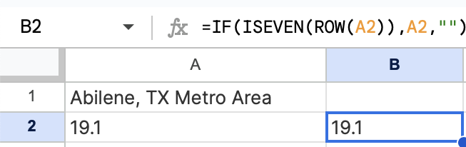
Getting the data
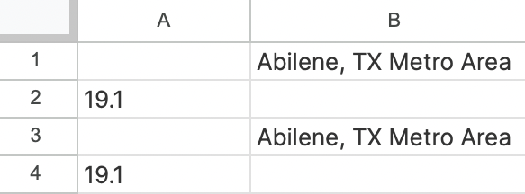
I had problems downloading the file from the Census website, so I manually copied and pasted the values into Excel. But it was all pasted in one column – with commute values in every other row. To fix this, I:
- Moved the time values to another column with
=IF(ISEVEN(ROW(A1)),A1,""), - Moved the metro values to the third column with
=IF(ISODD(ROW(A1)),A1,""), - Replaced these formulas with values and deleted the original broken column,
- Moved column A up by one cell,
- Filtered out the empty cells,
- Dropped duplicates,
- Split the geographic colummn by City and State,
- Removed the second and third towns in metropolitan area names.
1
2
| commute = pd.read_csv('Data/commute.csv')
cities = merge_frames(commute)
|
Location
Latitude and longitude for mapping data with Plotly and Tableau. Data from SimpleMaps.
1
2
| geodata = pd.read_excel('Data/geodata.xlsx')
cities = merge_frames(geodata)
|
Categorical Variables and State Names
Lastly, we need to add two categorical variables for the future analysis, namely:
- Region – for this I’ll use the Census division of South, Midwest, Northeast, West;
- Size rank – whether a city is considered large, small, or in between. Also, I want to change the two-letter state abbreviations to full names, because it looks nicer.
First, I ask ChatGPT to generate two dictionaries. One with two-letter state names as keys and full names as values and one with regions as keys and full names as values.
Then I’ll modify the DataFrame using these dictionaries.
The Region Category
1
2
3
4
5
6
7
8
9
10
11
12
| # Import generated dictionaries
from state_dicts import state_names, us_regions
# Create a new list by matching values from the State column with state_names dictionary
state_list = list(cities.State)
new_state_list = [state_names[state_list[i]] for i in range(len(state_list))]
# Change values in the State column
cities['State'] = new_state_list
# Create a new column with region information by iterating through us_region dictionary and the State column, and matching the values
region_list = [next(key for key, val in us_regions.items() if x in val) for x in cities['State']]
cities['Region'] = region_list
|
The Size Category
There is no single definition of what constitutes a large, medium, or small metropolitan area. The definition varies depending on the context. Given the data, for the purposes of this project, the size of a metropolitan area is defined as follows:
- Large — over one million people,
- Mid-sized — over 250 thousand and less than one million people,
- Small — less than 250 thousand people.
1
| cities['Size'] = pd.cut(cities['Population'], bins=[0, 250000, 1000000, np.inf], labels=['Small', 'Mid-Sized', 'Large'])
|
1
2
3
| # Rearrange the columns
cols = list(cities.columns)
cities = cities[cols[:2] + cols[-2:] + cols[2:7] + cols[11:14] + cols[7:11] + cols[14:16]]
|
1
2
| # Final version of the DataFrame before cleaning
cities.sample(5)
|
| City | State | Region | Size | Population | AvgRent | MedianRent | UnempRate | AvgIncome | CostOfLiving | PriceParity | CommuteTime | MedianAQI | WalkScore | BikeScore | TransitScore | Latitude | Longitude |
|---|
| 225 | Redding | California | West | Small | 182155.0 | 1445 | 1081.0 | 4.1 | 54972.0 | 108.7 | 99.40 | NaN | 44.0 | NaN | NaN | 1.8 | 40.5698 | -122.3650 |
|---|
| 249 | Blacksburg | Virginia | South | Small | 166378.0 | 1926 | 924.0 | 2.5 | 44904.0 | 94.5 | 92.19 | 20.5 | 40.0 | NaN | NaN | 2.0 | 37.2300 | -80.4279 |
|---|
| 140 | Tallahassee | Florida | South | Mid-Sized | 384298.0 | 1360 | 1086.0 | 2.2 | 52279.0 | 96.4 | 94.97 | 22.6 | 43.0 | NaN | NaN | 2.6 | 30.4551 | -84.2527 |
|---|
| 263 | Traverse City | Michigan | Midwest | Small | 153448.0 | 1592 | NaN | NaN | NaN | 99.6 | NaN | 22.5 | 39.0 | NaN | NaN | NaN | 44.7546 | -85.6038 |
|---|
| 365 | Casper | Wyoming | West | Small | 79955.0 | 1122 | 787.0 | 3.9 | 70175.0 | 94.2 | 91.34 | NaN | 43.0 | NaN | NaN | 1.8 | 42.8420 | -106.3208 |
|---|
Cleaning Data
Checking for null values
First, we find the non-standard missing values – the ones that are undetectable by pandas because they don’t look like NaN.
To do this, we loop through the rows of numeric columns and try to convert values to int. If that’s not possible, then there’s missing data.
1
2
3
4
5
6
7
8
9
10
11
12
13
14
15
16
17
18
19
20
21
22
23
24
25
26
| # Select only numeric columns
cols_to_loop = cities.columns[4:]
# Dictionary to store all non-standard missing values and their amounts
missing_dict = dict()
# Loop though each row
for i, row in cities.iterrows():
# And then though each column
for col in cols_to_loop:
# Try convert values of the original DF to integers
try:
cities.at[i, col] = float(cities.at[i, col])
# If that's not possible then it's missing data
except ValueError:
# If new string encountered, add to dictionary, otherwise update count
if row[col] in missing_dict:
missing_dict[row[col]] += 1
else:
missing_dict[row[col]] = 1
# Replace this string with NaN
cities.at[i, col] = np.nan
missing_dict
|
Drop Rows with Lots of NaN Values
Our table has too many missing values for the simple reason that each CSV we loaded had a different set of cities. There are 67 cities out of 456 with all the rows filled.
1
2
| # Number of cities with all the rows filled
cities.loc[cities.isna().sum(axis=1) == 0, 'City'].count()
|
We’ll delete cities with more than half of the variables missing. They are all quite small, with only a dozen metro areas having more than 100,000 inhabitants.
1
2
| dropped_cities = (cities.isna().sum(axis=1) >= 6)
cities = cities.loc[~dropped_cities].reset_index(drop=True)
|
Check If All the Data Types Are Correct
1
2
3
4
5
6
7
8
9
10
11
12
13
14
15
16
17
18
19
20
21
22
23
24
25
| <class 'pandas.core.frame.DataFrame'>
RangeIndex: 344 entries, 0 to 343
Data columns (total 18 columns):
# Column Non-Null Count Dtype
--- ------ -------------- -----
0 City 344 non-null object
1 State 344 non-null object
2 Region 344 non-null object
3 Size 344 non-null category
4 Population 344 non-null float64
5 AvgRent 344 non-null int64
6 MedianRent 338 non-null float64
7 UnempRate 335 non-null object
8 AvgIncome 344 non-null float64
9 CostOfLiving 335 non-null float64
10 PriceParity 343 non-null float64
11 CommuteTime 289 non-null float64
12 MedianAQI 302 non-null float64
13 WalkScore 74 non-null float64
14 BikeScore 74 non-null float64
15 TransitScore 344 non-null float64
16 Latitude 344 non-null float64
17 Longitude 344 non-null float64
dtypes: category(1), float64(12), int64(1), object(4)
memory usage: 46.3+ KB
|
Unemployment Rate and Transit Score are seen as objects by pandas, although they should be floating po
1
2
| cities['UnempRate'] = cities['UnempRate'].astype(float)
cities['TransitScore'] = cities['TransitScore'].astype(float)
|
Final Version of the Table
| City | State | Region | Size | Population | AvgRent | MedianRent | UnempRate | AvgIncome | CostOfLiving | PriceParity | CommuteTime | MedianAQI | WalkScore | BikeScore | TransitScore | Latitude | Longitude |
|---|
| 9 | Boston | Massachusetts | Northeast | Large | 4941632.0 | 3419 | 2368.0 | 2.9 | 92290.0 | 132.6 | 109.69 | 31.2 | 44.0 | 82.8 | 69.4 | 5.0 | 42.3188 | -71.0852 |
|---|
| 23 | San Antonio | Texas | South | Large | 2558143.0 | 1441 | 1138.0 | 3.3 | 53648.0 | 92.7 | 96.38 | 26.7 | 51.0 | 36.9 | 44.5 | 4.5 | 29.4632 | -98.5238 |
|---|
| 74 | Stockton | California | West | Mid-Sized | 779233.0 | 1915 | 1257.0 | 5.2 | 57783.0 | 113.6 | 104.61 | 33.3 | 43.0 | 43.7 | 52.4 | 3.0 | 37.9765 | -121.3109 |
|---|
| 296 | Cleveland | Tennessee | South | Small | 126164.0 | 1328 | 754.0 | 3.1 | 45404.0 | 89.5 | 88.02 | NaN | NaN | NaN | NaN | 0.0 | 35.1817 | -84.8707 |
|---|
| 130 | Savannah | Georgia | South | Mid-Sized | 404798.0 | 1744 | 1204.0 | 2.5 | 53570.0 | 97.3 | 95.42 | 24.3 | 39.0 | NaN | NaN | 2.5 | 32.0286 | -81.1821 |
|---|
| 79 | Lakeland | Florida | South | Mid-Sized | 725046.0 | 1674 | 1010.0 | 2.7 | 43556.0 | 96.4 | 96.17 | 25.7 | 41.0 | NaN | NaN | 1.6 | 28.0557 | -81.9545 |
|---|
| 199 | Lake Charles | Louisiana | South | Small | 222402.0 | 1083 | 833.0 | 3.0 | 51080.0 | 89.4 | 90.24 | NaN | 44.0 | NaN | NaN | 0.9 | 30.2010 | -93.2111 |
|---|
| 53 | Urban Honolulu | Hawaii | West | Large | 1016508.0 | 2428 | 1892.0 | 3.4 | 63912.0 | NaN | 114.74 | 29.0 | 29.0 | 65.7 | 51.0 | 6.4 | 21.3294 | -157.8460 |
|---|
| 62 | Albany | New York | Northeast | Mid-Sized | 899262.0 | 1475 | 1166.0 | 2.5 | 67788.0 | 100.1 | 99.16 | 23.4 | 39.0 | NaN | NaN | 3.6 | 42.6664 | -73.7987 |
|---|
| 75 | Greensboro | North Carolina | South | Mid-Sized | 776566.0 | 1421 | 981.0 | 3.6 | 51872.0 | 91.0 | 92.82 | 22.1 | 43.0 | 29.4 | 32.2 | 1.8 | 36.0956 | -79.8271 |
|---|
Create an Excel and CSV documents from our final DataFrame.
1
2
| cities.to_excel('us_cities.xlsx')
cities.to_csv('us_cities.csv')
|
Conclusion
By the end of this project, we have a dataset of American cities with a dozen variables. We gathered this data from open sources and explained how each variable was collected and calculated. We also assigned two categories (Region and Size) based on the data.
At first, we did a lot of cleaning in Python to be able to merge the data with the final dataset (AvgRent, MedianRent, UnempRate columns). The latest data was much cleaner, and we pre-processed it in Excel to save time. I usually just separated the columns with a delimiter and formatted the numeric values.
Then we cleaned the data: found and replaced missing data, dropped raws with lots of missing values, and corrected data types. This dataset can be found on this project’s GitHub page. I have also uploaded it on Kaggle.
We delve into this data with data analysis in the second part.