Introduction
Data. In this project, we are conducting an A/B test for an e-commerce website. This data was downloaded from Kaggle with no context as to where the data came from and what it represents. The ‘landing_page’ column suggests that we’re dealing with two versions of a landing page that appears after a user clicks on a link in an email or an ad.
Hypothesis. The null hypothesis is that the new webpage design is not statistically different from the old one. To reject the null hypothesis, the probability of obtaining the observed results should be less than or equal to 0.05 (the alpha value).
Metrics. The “converted” column shows whether a user took some action after landing on a page. This could be adding an item to the shopping cart or making a purchase.
Load and Explore Data
1
2
3
4
5
6
| import math
import numpy as np
import pandas as pd
import scipy.stats as stats
import statsmodels.stats.api as sms
from statsmodels.stats.power import tt_ind_solve_power
|
1
2
3
| df = pd.read_csv('ab_data.csv')
countries = pd.read_csv('countries.csv')
print(countries.country.unique())
|
1
2
3
| # Merge two data sets and display it
df = pd.merge(df, countries, how='left', on='user_id')
df.head(5)
|
| user_id | timestamp | group | landing_page | converted | country |
|---|
| 0 | 851104 | 11:48.6 | control | old_page | 0 | US |
|---|
| 1 | 804228 | 01:45.2 | control | old_page | 0 | US |
|---|
| 2 | 661590 | 55:06.2 | treatment | new_page | 0 | US |
|---|
| 3 | 853541 | 28:03.1 | treatment | new_page | 0 | US |
|---|
| 4 | 864975 | 52:26.2 | control | old_page | 1 | US |
|---|
There are two columns in the dataset that look like duplicates. The “group” column contains “control” and “treatment” groups, and the “landing_page” has “old_page” and “new_page” values. The first thing we need to do is check for inconsistencies (i.e. having “old_page” in the treatment group or “new_page” in the control group).
1
| pd.crosstab(df.group, df.landing_page)
|
| landing_page | new_page | old_page |
|---|
| group | | |
|---|
| control | 1928 | 145274 |
|---|
| treatment | 145315 | 1965 |
|---|
There are 1928 incorrect entries in the control group and 1965 in the treatment group out of a total of 294480.
These inconsistencies could be intentional (as part of the experimental design) or caused by implementation errors. If I encountered this problem in a real-world project, I would consult with the team to find a reason before working with the data. Now, given our goals and the large size of the set, we can safely delete these values and move on.
1
2
3
4
| # Filter out and delete inconsistent rows
wrong_entries_control = (df.group == 'control') & (df.landing_page == 'new_page')
wrong_entries_treatment = (df.group == 'treatment') & (df.landing_page == 'old_page')
df = df.loc[~(wrong_entries_control | wrong_entries_treatment)]
|
Now, we can split the data into two groups.
1
2
3
| # Split by groups
group_A = df[df['group'] == 'control']
group_B = df[df['group'] == 'treatment']
|
Choose the sample size
Each group has approximately 145,000 values. Running a test of this size would be too costly and slow. To choose the sample size, we need the following parameters:
- Alpha: Determined by the significance level (is the probability that the event could have occurred by chance, 0.05 in our case);
- Power: Probability of finding a statistical difference between two groups given that there is some difference (0.8 if we follow convention);
- Baseline Conversion Rate : How many visitors were “converted”. Calculted by dividing the number of such visitors by the total number of visitors.
- Minimum Detectable Effect: The lift by which another design solution makes a difference. We want to see at least 14% conversion versus 12% for the old design.
- Ratio: The ratio of the tratment sample to the control sample.
Knowing the actual baseline conversion rate and the desired lift, we can calculate the effect size, or Cohen’s d.
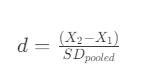
- Effect Size: In simple terms, measures the strength of the relationship between two groups. To calculate it, we divide difference between two means (i.e. conversion rates) by the pooled standard deviation.
- The pooled standard deviation required for Cohen’s d, is calculated as follows:
1
2
3
4
5
6
7
| ## Defining parameters
alpha = 0.05
power = 0.8
# Calculating baseline conversion rate, that is equal 0.12
x1 = round(sum(group_A['converted'] == 1) / len(group_A), 3)
# We want this rate to be at least 0.14
x2 = x1 + 0.02
|
We can find the effect size in two ways – by plugging all the parameters into the formula, or with a Python function.
Either way, we get a value of about 0.0595. Negative/positive signs don’t matter here, as we take the absolute value of the Cohen’s d for further calculations.
1
2
3
4
5
6
7
8
9
10
11
| ## Effect size, Method 1
# Find variance that is the standard deviation squared
base_var = x1 * (1 - x1)
target_var = x2 * (1 - x2)
# Find the effect size
effect_1 = (x2 - x1) / math.sqrt((base_var + target_var) / 2)
print(round(effect_1, 4))
## Effect size, Method 2
effect_2 = sms.proportion_effectsize(x1, x2)
print(round(effect_2, 4))
|
To find the sample size, we can use two different methods from the statsmodel library. The tt_ind_solve_power() function is more versatile, while the NormalIndPower().solve_power() is simpler and just ideal for our case.
1
2
3
4
5
6
7
8
9
10
11
12
13
14
15
16
17
18
| ## Sample size, Method 1
sample_size = int(sms.NormalIndPower().solve_power(
effect_size=effect_1,
alpha=alpha,
power=power,
ratio=1
))
print(sample_size)
## Sample size, Method 2
sample_size = int(tt_ind_solve_power(
effect_size=effect_1,
nobs1=None,
ratio=1,
alpha=alpha,
power=power,
alternative='two-sided'))
print(sample_size)
|
Testing
There are many ways to do A/B testing in Python with our data. I chose the chi-squared test for its simplicity (after all, our case is not the most difficult one). Also, I’ll try a popular and more versatile bootstrap test.
1
2
3
| # Sample
sample_A = group_A.sample(sample_size, random_state=1)
sample_B = group_B.sample(sample_size, random_state=1)
|
1
2
3
4
| # Calculate means and standard deviations for our samples
print(sample_A['converted'].agg([np.mean, np.std]))
print()
print(sample_B['converted'].agg([np.mean, np.std]))
|
1
2
3
4
5
6
7
| mean 0.120631
std 0.325735
Name: converted, dtype: float64
mean 0.114092
std 0.317959
Name: converted, dtype: float64
|
Chi-square test
Basically, the chi-squared test compares the observed frequencies (i.e. how often a categorical value is in the data) of different categories in a contingency table with the frequencies we would expect to see if there were no association between the variables. The test evaluates whether the observed frequencies are significantly different from the expected frequencies, which is an indication of a potential relationship.
First, we create a contingency table using the pandas.crosstab function. Second, we use the chi2_contingency function from scipy to find a p-value.
1
2
3
| both_groups = pd.concat([sample_A[['country', 'group', 'converted']], sample_B[['country', 'group', 'converted']]])
ab_contingency = pd.crosstab(both_groups.group, both_groups.converted)
print(ab_contingency)
|
1
2
3
4
| converted 0 1
group
control 3900 535
treatment 3929 506
|
1
2
3
| chi2_statistic, p, dof, expected = stats.chi2_contingency(ab_contingency)
print(f'The contingency table if there were no association:\n{expected}\n')
print(f'P-value: {round(p, 2)}.')
|
1
2
3
4
5
| The contingency table if there were no association:
[[3914.5 520.5]
[3914.5 520.5]]
P-value: 0.36.
|
The p-value of 0.36 is a lot larger than the significance threshold of 0.05. It means there is no significant difference beween two landing page designs.
Bootstrap test
Another great way to test our hypothesis is a bootstrap. This could be done with the scipy.stats.bootstrap function, but for demonstration purposes, we’ll calculate the p-value ‘by hand’ (I also love the whole iteration thing in this code).
The p-value is larger than in the previous test, but is still well above the significance threshold.
1
2
3
4
5
6
7
8
9
10
11
12
13
14
15
16
17
18
19
20
| observed_diff = np.mean(sample_B.converted) - np.mean(sample_A.converted)
n_iterations = 1000
# Array to store bootstrap sample statistics
bootstrap_stats = np.zeros(n_iterations)
for i in range(n_iterations):
# Generate bootstrap samples
treatment_sample = np.random.choice(sample_B.converted, size=len(sample_B.converted), replace=True)
control_sample = np.random.choice(sample_A.converted, size=len(sample_A.converted), replace=True)
# Calculate test statistic for the bootstrap sample
bootstrap_diff = np.mean(treatment_sample) - np.mean(control_sample)
# Store the bootstrap statistic
bootstrap_stats[i] = bootstrap_diff
# Count the proportion of bootstrap statistics that are greater than or equal to the observed difference (-0.00654 in this case)
p = np.mean(bootstrap_stats >= observed_diff)
print(f'P-value: {round(p, 2)}')
|
Other factors
Total Time Spent on the Website
There are two variables that can give more insight into user behavior on the site.
The first one is a timestamp. There is no information in the dataset about what this column represents. My guess is that it is the total time a user spent on the site, in minutes and seconds.
1
2
3
| # Convert 'timestamp' to minutes
df['total_minutes'] = df['timestamp'].apply(lambda x: round(float(x[:2]) + float(x[3:]) / 60, 2))
df.head()
|
| user_id | timestamp | group | landing_page | converted | country | total_minutes |
|---|
| 0 | 851104 | 11:48.6 | control | old_page | 0 | US | 11.81 |
|---|
| 1 | 804228 | 01:45.2 | control | old_page | 0 | US | 1.75 |
|---|
| 2 | 661590 | 55:06.2 | treatment | new_page | 0 | US | 55.10 |
|---|
| 3 | 853541 | 28:03.1 | treatment | new_page | 0 | US | 28.05 |
|---|
| 4 | 864975 | 52:26.2 | control | old_page | 1 | US | 52.44 |
|---|
1
2
3
4
5
| # Show average minutes for all scenarios with a pivot table
df.pivot_table(index=['converted'],
columns=['group'],
values=['total_minutes'],
aggfunc='mean')
|
| total_minutes |
|---|
| group | control | treatment |
|---|
| converted | | |
|---|
| 0 | 30.099602 | 30.019013 |
|---|
| 1 | 29.954144 | 30.070834 |
|---|
Findings. I see no point in continuing with the time variable. The pivot table of minute means shows no difference in conversion rates between the groups. Also, we can only assume that this column represents the time spent on the website, as we’ve got no data dictionary.
Countries
Finally, let’s take a look at the countries data set.
The pivot table shows the largest difference among Canadian users, and the smallest in the US.
1
2
3
4
| both_groups.pivot_table(index=['country'],
columns=['group'],
values=['converted'],
aggfunc='mean')
|
| converted |
|---|
| group | control | treatment |
|---|
| country | | |
|---|
| CA | 0.115741 | 0.093750 |
|---|
| UK | 0.127773 | 0.112029 |
|---|
| US | 0.118370 | 0.116505 |
|---|
To not repeat yourself and to show another approach to A/B testing, we’ll run one of the following tests on the data, filtered by country:
- Two-sample t-test if the data is normally distributed,
- Mann-Whitney U test if not.
1
2
3
| # Check the normality with the Shapiro-Wilk W test for both samples
normality_pvalues = (stats.shapiro(sample_A.converted)[1], stats.shapiro(sample_B.converted)[1])
print(normality_pvalues)
|
Since data is not normal, we’ll run the nonparametric Mann-Whitney U test. This test compares two independant samples to determine if they come from the same population.
1
2
3
4
5
6
| # Create filters to access the rows with selected countries
countries_list = ['US', 'UK', 'CA']
for country in countries_list:
country_filter = both_groups.country == country
u, p = stats.mannwhitneyu(sample_A.loc[country_filter]['converted'], sample_B.loc[country_filter]['converted'])
print(f'P-value for {country}: {p}')
|
1
2
3
| P-value for US: 0.8198610487339111
P-value for UK: 0.25442017080004864
P-value for CA: 0.43604924692614255
|
Findings. Despite some differences in conversion rates when the data is broken down by country (e.g. users from the UK were converted 1% more often), the test shows that this difference is not significant.
Conclusion
The hypothesis that two webpage designs are not different in terms of the conversion rate was failed to be rejected. It means that there was no difference in user behavior when landing on an old or new page. To test this, we used the chi-square test (Python function) and the bootstrap test (“by hand”). Since the data size was too large, we found a sample size with two methods. Lastly, we checked the influence of other factors such as time and country, but also found no significant effect.